Overview
In closed capture models, the primary interest and goal is to estimate abundance at a single point in time. These methods were characterized by a strict assumption of population closure- no births, deaths, or movement into or out of the study area. Sometimes our interest moves beyond a point estimate of abundance and we are interested in estimating births, deaths, and how abundance changes over time. To do that, we need to use open population models.
As the name implies, we no longer need to assume population closure in between capture events. Animals can be born and die (but ideally don’t leave the study area). And it’s these processes of recruitment and survival (or apparent survival) that we are interested in learning more about. There are several open population capture recapture models. There are differences among them but they generally are suitable for use when working with an open population. All provide some information about the processes that make a population open, births and deaths, and generally some kind of information about abundance or at least population growth rates. In order to do so, they come with their own set of assumptions. The big picture assumptions/requirements are generally the same as closed captures like:
- Study area is constant
- Tags are read correctly
- Require > 1 marking occasion
If you recall from closed captures, there were both “full” or “unconditional” likelihood methods as well as “conditional” likelihood methods. Open models have a have similar organization. Here, those terms are synonymous with methods that estimate abundance versus those that estimate parameters such as recruitment or population growth, respectively. Because of that, for unconditional likelihood methods, we have an assumption that hasn’t been relevant since Lincoln-Petersen:
- Catchability among marked and unmarked individuals is equivalent.
This is a critical assumption for open models. In closed captures, we could account for trap-happy or trap-shy responses by animals. However, when using an unconditional likelihood open population model, you cannot.
Additionally, because we are now modeling new parameters, there are novel assumptions, namely:
- Survival among marked and unmarked individuals are the same.
This holds regardless of whether you use a full or conditional likelihood. While catchability is important if you are trying to estimate abundance, inference about other quantities of interest from open models such as population growth cannot be valid if marked individuals differ somehow from unmarked individuals.
Open capture-recapture models
Now, we’ll cover the most common and simple types of open capture-recapture models and how and when they might be used.
The Cormack-Jolly-Seber (CJS) model is one of the simplest open models and it doesn’t really fit in with the other models we’re going to discuss here. That is because CJS only estimates two parameters: apparent survival (\phi) and recapture probability (p). It warrants discussion here because all of the other models, variations of something called Jolly-Seber (JS) models, use the CJS in their calculations.
You may notice that we called \phi apparent survival, not survival. This is because we never observe dead animals in these types of studies. Thus, when we don’t capture an animal again, we aren’t sure if it is because we just don’t catch it, it died, or it moved out of our study area (permanent emigration). Permanent emigration is indistinguishable from death in CJS. Thankfully, if no emigration out of the study area occurs, then \phi is the same as true survival.
CJS is a type of conditional likelihood model. It’s conditional because we don’t much care how individuals are marked initially, we are only concerned about recapture probability and apparent survival after the initial capture. This means that some of the assumptions that will still hold for JS models, aren’t relevant here.
Typically for a CJS study, individuals marked and released on several different occasions across years or whatever interval you are trying to estimate survival. However, you don’t always need to have multiple marking/release occasions (such as a translocation study) but your ability to estimate survival as time goes on (and precision) will suffer if you do not because fewer animals are likely to be alive the farther you are in time from the release period. It’s just not necessary, unlike JS models.
Also unlike JS models, CJS doesn’t need to assume the study area stays the same size. If you start capturing animals in new areas, you may wish to test if survival differs among areas, but it won’t otherwise affect your estimates of p and \phi. You don’t technically have to assume that \phi is the same among marked and unmarked animals-but we generally do. If we did not, what use would our estimate of \phi be?
The Jolly-Seber model is both a specific formulation of an open capture-recapture model and a “family” of models. All models in the JS family represent the same fundamental process, just with different tweaks and assumptions.
The original Jolly-Seber model was developed by Jolly and Seber separately and is considered a full or unconditional likelihood. It primarily used counts of newly marked individuals and recaptured individuals at multiple capture events through time to estimate capture/recapture probability (p), net entrants (B), survival (\varphi), and abundance (N). It’s generally not used anymore for a few different reasons, but perhaps most importantly, the estimate of “net entrants” to the population was often estimated as < 0, which is biologically impossible.
Still the general framework is to mark and release individuals at multiple points in time. While individual encounter histories can be recorded, the method can use aggregated counts of captures, recaptures, total releases, etc. You can look into the approach more on your own, we won’t go into it here.
Technically a full/ unconditional model, it’s hard to find out much on this parameterization because the paper is in an obscure “transactions” journal. It’s generally not recommended to be used because it usually doesn’t converge.
POPAN is one alternative parameterization or flavor of a Jolly-Seber Model. It’s chief advantage is it prevents the number of “net births/entrants” from ever being less than 0. It does this by estimating a “superpopulation” comprised of all individuals that will ever exist in the population. It then estimates an entry probability (b) while also estimating survival (\varphi) and capture probability (p). This approach can be useful when obtaining the number of individuals entering a population or existing in a population at any time point is desired.
It can be tricky to fit in practice if you try to fit complex time dependent models. This is important, because resulting abundance estimates are heavily dependent on accurate model structure for entry and capture probability. If the model for entry or catchability are incorrect, the resulting abundance estimate will be biased. Covariates for catchability, entry, and survival can be included, but not at the individual level because you don’t know the values for individuals before they enter the population and are caught.
The Link-Barker approach avoids some of the problems of POPAN, but at a cost. Like a CJS, Link-Barker does not attempt to account for the initial capture probability, it only cares about recapture after the initial event. Therefore, the Link-Barker model cannot estimate abundance or the number of entrants to a population. Instead, it estimates \varphi and f, fecundity (the number of new individuals that enter the population and survive to be captured per existing individual) as the main demographic parameters of interest. This approach is similar to the Pradel model, except it accommodates individuals that may die (or lose their markings) at capture. You can included covaraites on all the parameters, even individual level covariates.
There are several versions of a Pradel model that primarily differ in what parameters you are able to model or add covariates to, and what is estimated after-the-fact. A Pradel model includes \varphi, p in addition to f (like the Link-Barker model), and two new parameters, \lambda, the growth rate, and \gamma, seniority. The \gamma parameter is new and unique to Pradel models. It’s obtained by “running” the data as CJS model, but reversing the time order of capture events. The resulting parameter, \gamma, is now the probability that an individual captured at a given time, was in the population at the preceeding capture interval. From estimating this parameter with the data, you can then derive \lambda as: \lambda = \frac{\varphi}{\gamma}
and f as:
f=\lambda - \varphi
as implemented in MARK, you can only model two of the four demographic parameters (\lambda, \varphi,f,\gamma). There are actually 4 different variants of the Pradel model that differ in what parameters are directly modeled. Which to choose depends on your ultimate goal and interest, but perhaps the most important thing to understand is, because most of these parameters are can be expressed as a function of others, changing one or two (by adding covaraites) will force remaining parameters to behave a certain way. For example, if you set f to be constant and \varphi to change linearly with time, \lambda will be forced to change linear with time, opposite of the change in \varphi. The upshot is you need to be careful and if this is an approach you think you may want to implement, you should consult one of the biometricians.
Final thoughts
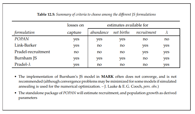
Different types of Jolly-Seber models, borrowed from the MARK manual.
Open population models are a useful tool for moving beyond the estimation of simple abundance and permit the estimation of other important demographic parameters. They can be difficult to fit in practice because results can be sensitive to how you construct the model (time dependence, covariates, etc.) Many of these issues are addressed with the Robust Design, which can be used in conjunction with all of the above models and has generally superseeded these more simple open models for free-ranging animal populations(with the exception of the CJS model). Still, the open models described here can be useful and probably see more use in applications beyond their initial purpose such as modeling hunter purchasing patterns or stopover behavior of migrating birds. The many different versions of open population models, particularly Jolly-Seber models