Time To Event and Known-fate (Survival) Analyses

Interval Censoring

The most common method of censoring is interval censoring. This is where you don’t know the exact event time, just that occurred sometime during an interval during the observation. So unless you are checking nests or your radio-marked individuals every day, you will have interval censored data. If you are fitting a GLM with a logit link, you probably dealt with interval censoring by using the logistic exposure link or another technique (like a cloglog link + offset). If you are familiar with Program MARK and have used the known-fate module there, the concept of interval censoring might seem confusing (it is for me at least) because, if you lose track of an individual, you code an interval as ‘00’ to indicate an individual was missing, and thus, censor that time period. They refer to it as interval censoring, but it’s not the same “interval censoring” as is mentioned in most other texts regarding TTE or survival analyses. It’s more accurately called interval truncation and DeCesare et.al (2015⁵) give a good explanation. It’s an artifact of Program MARK using a model that does not permit interval censoring. They even tell you that you should use their nest-survival module if you have interval censoring.

Compare that to TTE analysis or almost any other analysis we’ll use where interval censoring is allowed. In this, you do not need to drop these observations. If the animal is observed detected dead later on, the interval censoring handles the uncertainty as to when mortality occurred. If you observe them alive later you know they survived. If you never encounter them dead or alive again, it’s just right censoring, and you are relying on the assumption that censoring is not informative. This also requires that the probability of detecting an individual doesn’t depend on their fate-the probability of finding that individual that went missing is the same, regardless if you are finding them dead or alive.

Right Censoring and informative censoring

If you lose track of an individual and never find them (alive or dead) or they haven’t died yet when the study ends, this is right-censoring. In the latter case, it’s called fixed censoring, whereas the former, it’s assumed random. That is, dying doesn’t cause you to loose track of an individual. If this censoring is informative (radio transmitters fail because they are destroyed by cars/people/predators) then your survival estimate will be biased. This is true regardless if you analyze the data in a TTE framework or a logistic regression framework. If it is random (or at least nearly) then it doesn’t matter. If you do lose track of a lot of individuals without knowing their fate, it’s recommended you don’t use an approach that relies on accurately knowing it.

Left Censoring and Truncation

Left censoring doesn’t make sense in a survival analysis, it means the event of interest occurred before that individual became part of the study. This is nonsense is it’s death. Left censoring undoubtedly occurs in our data sets, but there is nothing we can typically do, statistically speaking, to account for it. What we typically have in our data sets is truncation.

Left-truncation applies to individuals not observed from their origin time, We experience this all the time with wildlife data; individuals have to survive long enough for us to capture them.

Truncation can be accommodated (in a TTE analysis or a GLM) if you specify a time at capture in a logit model or an entry time (relative to origin). This is where it gets hard for me to wrap my head around. The whole issue of left trunction or censoring only really makes sense if you really do have an “origin time”, otherwise we often just get taught ways to avoid having to deal with this. Hazard models accommodate left truncation by only considering the interval for when the individual was first observed. In a GLM, we generally would treat it as “heterogeneity” and deal with it by including an appropriate covariate, such as age-at-capture, and then maybe including age as a time-varying covariate.

Clearly this doesn’t correct for the fact we might not be observing individuals in some age/stage classes. There really isn’t a statistical approach to “fix” this-it’s a sampling issue. That’s why we generally talk about survival estimates for specific age-classes or at stages.

GLM approaches -Logit link

When talking about survival or a time-to event analysis it’s helpful to start talking about using a GLM to estimate survival (or mortality) because it’s probably what most folks are familiar with. The first big difference is that using a GLM, you’re modeling the probability of the event occurring over some interval, not how long before it occurs. We generally use this approach (as opposed to a TTE method), because we really don’t have the ability to define an origin time, typically because individuals are entering and leaving the study at varying time points and/ or because we can’t accurately age individuals.

In this approach, your data is probably a table with, at minimum, rows equal to the number of individuals x the number of intervals and a column indicating if that individual survived or died during that interval (e.g. 1/0). If your intervals are regular and equal in length you can use generic, built-in methods for estimating survival (e.g. logit link). If you are interested in modeling survival as a function of time (age, day of year), you typically deal with it by using a interval-specific covariate. Left truncation can be dealt with in this way, interval truncation can be handled by omitting those intervals where you were unable to verify the status of an individual (but might not be necessary), and right censoring is handled implicitly by an individual no longer appearing in the records.

If the checks are at irregular intervals, or you experience more than a trivial amount of interval truncation, then you are better off accounting for the variable length of time in each interval using the logistic exposure method.

Kaplan-Meier

Kaplan-Meier is called a non-parametric method because any of the quantities you describe (cumulative survival, period survival) are obtained by simple arithmetic where:

$$S_t=\frac{N_{alive\ at\ t}}{N_{alive\ t-1}}$$

You’re not using a linear model to estimate parameters. If you only use discrete covariates, then a logit model as described above is equivalent to a Kaplan-Meier estimate. However, a logit model gives you more flexibility, namely in the types of covariates you can include. Furthermore, Kaplan-Meier estimates assume there is no interval censoring. It’s generally your best bet if you don’t have very many individuals in your data set.

Plots of Kaplan-Meier estimates typically show cumulative survival probability as a function of time in a stair-step pattern. Note that this is not implying that survival probability varies with time. Kaplan-Meier estimates survival at each time step, but it is visualized as the proportion of individuals remaining at time T, which is equivalent to $S^T$, where $S$ is the 1-unit survival probability.

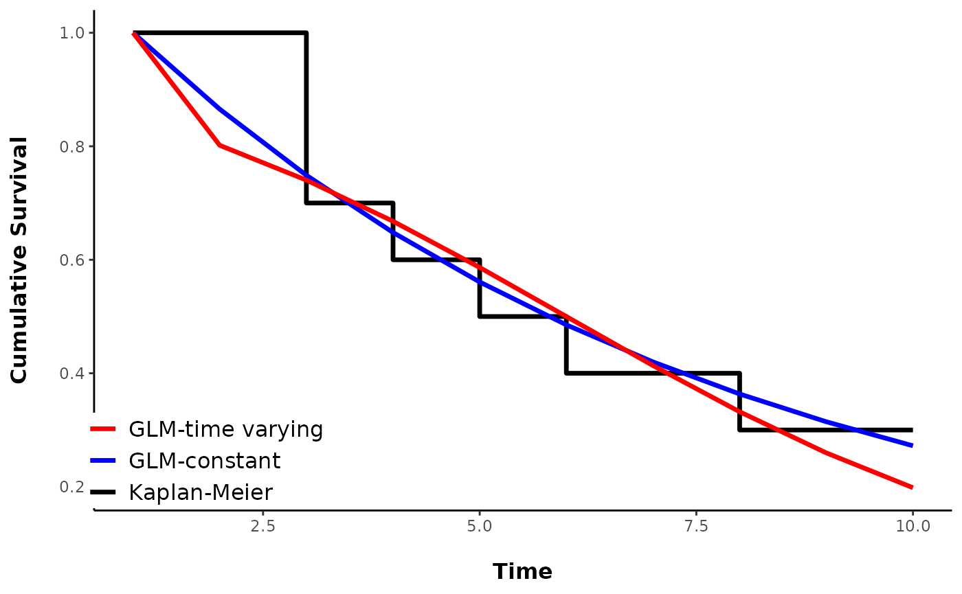
You can see that the GLM- constant survival estimates the cumulative survival probability as being lower than observed in the data, until the end, which is what the KM estimate shows. Nevertheless, they all produce the same average daily survival rate. The GLM that allowed time-varying survival is a better approximation of the KM curve, but also may just be overfitting, as the data for the plot were simulated using a constant survival probability.

Log-Log link

An alternative to using logit-link regression is to use a log-log link or:

$$S=exp(-exp(X\beta))\\ and\ the\ inverse\\ X\beta=log(-log(S))$$

where $S$ is the survival probability and $X\beta$ is the linear predictor. This approach gives the same interpretation (hazard ratios) of the $\beta_k$ regression coefficients as in proportional hazard models. Often this is preferable to using the logit link because hazards ratios (the relative difference in mortality) don’t change whether your model is talking about weekly, monthly, or annual survival. Odds ratios will differ, which may be just confusing or worse, misleading. In R, you have to use the complementary log-log link, which is equivalent to replaceing $S$ with $M$, as that is what $X\beta$ predicts. In R, you still code your data as 1=alive, 0=dead, but you are essentially modeling the 0’s when using that data structure and the cloglog link.

Interval censoring can be accommodated when using the logit-link by using the logistic-exposure link, and including an offset for the number of exposure days in each interval when using the cloglog link.

Semi parametric

The semi-parametric hazard model is synonymous with Cox’s proportional hazard. It is not, however, the only version of a proportional hazard model. Cox gets his name attached because he came up with a slick way to estimate the regression coefficients of $\lambda_t$ without ever having to estimate $\lambda_0$, using a partial likelihood. People don’t really like trying to have to specify that baseline so it’s often preferable to use this approach. However, a true Cox’s proportional hazard model doesn’t work with interval censoring, so most applications will probably use a parametric hazards model. For example, if you have interval censoring and want to use a proportional hazard model, you will actually fit a parametric hazard model, using an exponential baseline hazard.

Important to note, like the cloglog link, you are modeling mortality, so negative coefficients (log-hazard ratios) mean a negative association with mortality. It’s also worth noting that without specifying some kind of distribution for the baseline hazard, you can only get a survivor curve by estimating the baseline with non-parametric methods. This is hard, and using a parametric, exponential model is the equivalent. So it’s more straightforward to just do that!

Parametric Hazards

Parametric hazards have you specify a distribution of the baseline hazard. Proportional hazards (PH), proportional odds (PO), and accelerated-failure-time (AFT) models are types all parametric TTE models. The difference in these models is:

• the link used to model the hazard
• whether the hazard changes through time.

Another way to see some of these connections is to re-write the time to event model as a linear function of the times of the event, not the hazard:

$$log(T)=\beta_0+\beta_1X_1+\beta_2X_2...+\sigma\epsilon$$

where an random disturbance term $\epsilon$ follows some distribution. Most software routines don’t estimate the variance of $\epsilon$ but hold it constant and estimate $\sigma$ as a scaling parameter instead. As is described in the Paul Allison SAS survival book, depending on the distribution you assume for $\epsilon$, there is a corresponding hazard function:

1. if $\epsilon$ is extreme-value (exponential distribution) and $\sigma$ is fixed at one then T is exponentially distributed and gives a hazard function:

$$log(h(t))=\beta_0^*+\beta_1^*X_1...\beta_k^*X_k$$

This is the functionally the same hazard model used in Cox’s PH but now with an intercept. This is an exponential model, or a constant hazard because nothing in here specifically models the hazard as a function of time. If we did have a term here that was a function of time, it would be an AFT model.

2. if $\epsilon$ is extreme-value (exponential distribution) but $\sigma$ isn’t fixed at 1, then T follows a Weibull distribution and, per the SAS survival book:

$$log(h(t))=\alpha\log(t)+\beta_0^*+\beta_1^*X_1...\beta_k^*X_k$$

This is now an AFT, depending on the parameter value of $\alpha$(see pp. 20-21 in SAS survival book). In this case, $\alpha$ controls how the hazard varies across time, ensuring that the event times T follow a Weibull distribution. If $\alpha$ is just 0, then the hazard is constant through time and we’re back at the exponential distribution.

Fun fact, the Weibull above is both and AFT and a PH model, and it’s the only form that can both. That’s because, in the equation above, you could think of the $\alpha\log(t)$ as a baseline hazard

Another way to write the Weibull hazard can be found in handout 9 here is as:

$$h(t)=\lambda p t^{p-1}\\ log(h(t))=log(\lambda)+log(p)+(p-1)log(t)\\ log(h(t))=\alpha\ log(t) +\beta_0^*+\beta_1^*X_1...\beta_k^*X_k$$

where $p$ is $\frac{1}{\sigma}$ from the $log(T)$ equation above. So it looks like the difference between the two resources is $\alpha \sim p-1$ and the value of log(p) seems to end up in the $\beta_0$?

Other forms include the Log logistic

$$h(t)=\frac{\lambda p t^{p-1}}{1+\lambda t^p}$$ which gives a proportional odds model. All of these are AFT models

Typically, however, when you are fitting an AFT model you’re not writing a linear model for the hazard, your linear model is for $log(T)$ and you coefficients will be expressed as their effect on survival time, not the hazard.

What makes a model an AFT and/or PH?

These graphs from here help visually demonstrate it, as does the lecture notes found here. The PH has proportional hazards, but not a constant hazard rate. In short a proportional hazards model assumes that the hazard ratio doesn’t change as time changes. A graph of the hazard of two groups over time would be parallel, with the peak in the hazard occurring at the same time. In the AFT, the hazard peaks earlier or later for one group. So it’s a difference of up/down vs. left/right. This is what is meant when books/slides say an AFT “stretches” time in an AFT.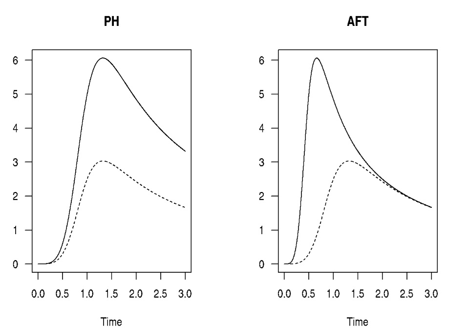

The other big difference is that when you fit an AFT model, you will code it up (or an existing package) where you put your linear model on survival time, not the hazard. This is because anything other than an exponential distribution gets really messy looking on the hazard scale. You can still derive it, but it’s more straight forward to write the linear model for $T$, not $h(t)$

Some AFT models are also PH models (e.g. Weibull), but most aren’t. They don’t need to be. The whole value of AFT models are for when you do not meet the proportional hazards assumption (i.e. the hazard ratio changes through time). Still in an AFT, you need to specify a baseline distribution for T.

• You typically won’t use an AFT with left truncation-why? You need those data to help fit the curve/ determine the appropriate shape of the baseline hazard. But if you want to be risky and specify one anyway, hope you’re right, you can “predict” outside of your sample the survival times of those individuals you never observed.

Because it’s hard to know what distribution to use for that baseline hazard (i.e. how does the hazard vary with time) it’s usually easier to turn an exponential PH model (which is not technically an AFT, as it has a constant baseline hazard) and throw in tricks to account for temporal variation or non-constant hazard ratios (see the slides from Reno). This approach works and is probably what you will end up doing most of the time, but as it gets more complicated (e.g. time-varying coefficients, piecewise exponential model), I think it feels a little too “Dr. Moreau” (clearly, Brando’s best film ever)

Analysis using a TTE hazards model

The model below a parametric model with an exponential distribution If you use a simple exponential function, your baseline hazard is constant and it will generally produce the same hazard ratios as a Cox PH model that doesn’t assume a baseline hazard.

library(nimble)

constant.model<-nimble::nimbleCode({
 gamma0~dflat()


  for (j in 1:records) {
    for (k in left[j]:(right[j]-1)) {
      UCH[j,k] <- exp(gamma0)
    }

    S[j] <- exp(-sum(UCH[j,left[j]:(right[j]-1)]))
    censored[j] ~ dbern(S[j])
  }

  for (i in 1:25) { #compute the survival function S0
    UCH0[i]<-exp(gamma0)
    CH0[i]<-sum(UCH0[1:i]) #sum the unit cumulative hazard to get the cumulative
                 #hazard (i.e prob of surviving day 1 to i, or S^2,S^3..S^i
    S0[i]<-exp(-CH0[i]) # transform to survival estimate to time i
  }
})



#define data and constants

nim.const<-list(records=nrow(tte.dat),
                left=tte.dat$left,
                right=tte.dat$right)
nim.dat<-list(censored=tte.dat$censor)


#inits

nim.init<-function(){list(
  gamma0=runif(1,-3,3)
)
}


constant.nimmod<-nimble::nimbleModel(code=constant.model,
                               constants=nim.const,
                               data=nim.dat,
                               inits=nim.init())

constant.nimmod$calculate()  # Check to make sure initial values are good.
                              #Should be a real number


constant.config<-nimble::configureMCMC(constant.nimmod)

# now is when you can specify different samplers and monitors
constant.config$addMonitors("CH0","UCH0","S0")


constant.build<-nimble::buildMCMC(constant.config)


#compile things

constant.comp<-nimble::compileNimble(constant.nimmod)

constant.mcmc<-nimble::compileNimble(constant.build, project=constant.comp)


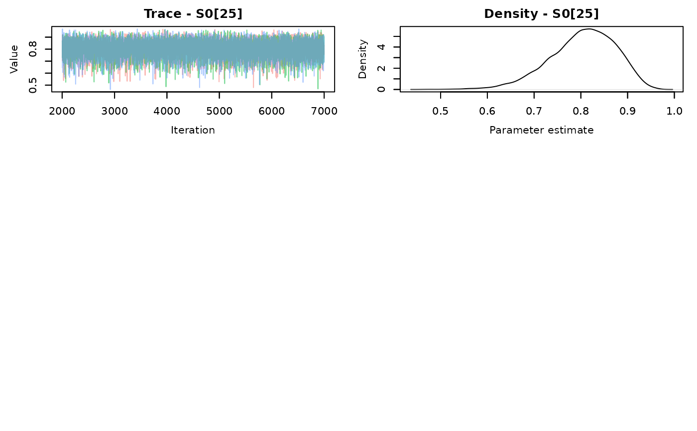
samples.constant<-nimble::runMCMC(constant.mcmc,
                             niter=5000,
                             nburnin = 1000,
                             nchains = 3)

##             mean        sd     2.5%       50%     97.5% Rhat n.eff
## gamma0 -4.153043 0.2928866 -4.76659 -4.136809 -3.627007    1  2676

The gamma parameter needs to be transformed back to survival. To do so, just exponentiate the value on the linear scale (in this case, just gamma, but it could include other terms). But this isn’t the surival probability, it’s the mortality probability. So the true transformation is:

$$S=1-exp(\gamma_0)\\ or\\ S=1-exp(\gamma_0+\gamma_1X_1+\gamma_2X_2...)$$

if there are covariates, where all the $\gamma_k$ are log hazard ratios (the equivalent of a $\beta$ in a GLM).

This means the estimated daily survival from the TTE model is 0.984.

Analysis using logistic exposure

#####   Create the link function
# Link function comes from Ben Bolker's page: https://rpubs.com/bbolker/logregexp

logexp <- function(exposure = 1) {
  ## hack to help with visualization, post-prediction etc etc
  get_exposure <- function() {
    if (exists("..exposure", env=.GlobalEnv))
      return(get("..exposure", envir=.GlobalEnv))
    exposure
  }
  linkfun <- function(mu) qlogis(mu^(1/get_exposure()))
  ## FIXME: is there some trick we can play here to allow
  ##   evaluation in the context of the 'data' argument?
  linkinv <- function(eta) plogis(eta)^get_exposure()
  logit_mu_eta <- function(eta) {
    ifelse(abs(eta)>30,.Machine$double.eps,
           exp(eta)/(1+exp(eta))^2)
  }
  mu.eta <- function(eta) {
    get_exposure() * plogis(eta)^(get_exposure()-1) *
      logit_mu_eta(eta)
  }
  valideta <- function(eta) TRUE
  link <- paste("logexp(", deparse(substitute(exposure)), ")",
                sep="")
  structure(list(linkfun = linkfun, linkinv = linkinv,
                 mu.eta = mu.eta, valideta = valideta,
                 name = link),
            class = "link-glm")
}

This link function needs to be in your GlobalEnvironment. Alternatively, it’s included as a function in the MDChelp package using ‘MDChelp::logexp()’

###########


mod.logexp<-glm(obs.ld~1,family=binomial(link=MDChelp::logexp(glm.dat$exposure)),
                data=glm.dat)

broom::tidy(mod.logexp)->parms.logit

parms.logit

## # A tibble: 1 × 5
##   term        estimate std.error statistic  p.value
##   <chr>          <dbl>     <dbl>     <dbl>    <dbl>
## 1 (Intercept)     4.02     0.280      14.4 1.00e-46

#DSR
plogis(parms.logit%>%
  pull(estimate))->dsr.logit

dsr.logit

## [1] 0.9824191

Analysis using the cloglog link and exposure time as an offset.

When back-transforming, we need the mean mean of the “exposure” variable.

mod.clog<-glm(obs.ld~1+offset(log(exposure)),
              family=binomial(link='cloglog'),
              data=glm.dat)


broom::tidy(mod.clog)->parms.clog

parms.clog

## # A tibble: 1 × 5
##   term        estimate std.error statistic  p.value
##   <chr>          <dbl>     <dbl>     <dbl>    <dbl>
## 1 (Intercept)    0.975    0.0745      13.1 4.36e-39

#calculate mean exposure
mu.exp<-glm.dat%>%pull(exposure)%>%mean()

data.frame(parms.clog[1,2]+log(mu.exp))%>%
  rename(lp=1)%>%
  mutate(dsr=1-exp(-exp(lp)))%>%
  pull(dsr)->dsr.clog

round(dsr.clog,digits=3)

## [1] 0.984

Now compare among the methods

See how they are all very similar to one another and less than 0.005 different than the data-generating value of 0.985? See how it only has a small effect on the cumulative survival probability $(DSR^{24})$ (24 survival periods to survive 25 days), which could just be sampling error. Very mindful, very demure.

Time-varying hazards model

To fit the time-varying hazards model, we fit the exponential model as above, and include a term to account for time. The method below just includes nest age as a covariate, but an alternative is to use a (improper) conditional autoregressive model. The iCAR model doesn’t try to specify any kind of functional relationship (like a linear model), but it can be more challenging to fit.

library(nimble)

time.model<-nimble::nimbleCode({
 gamma0~dflat()
  beta~dflat()
  
for(i in 1:24){
  age[i]<-beta*nest.age[i]
}
  for (j in 1:records) {
    for (k in left[j]:(right[j]-1)) {
      
      UCH[j,k] <- exp(gamma0+age[k])
    }

    S[j] <- exp(-sum(UCH[j,left[j]:(right[j]-1)]))
    censored[j] ~ dbern(S[j])
  }

  for (i in 1:24) { #compute the survival function S0
    UCH0[i]<-exp(gamma0+age[i])
    CH0[i]<-sum(UCH0[1:i]) #sum the unit cumulative hazard to get the cumulative
                 #hazard (i.e prob of surviving day 1 to i, or S^2,S^3..S^i
    S0[i]<-exp(-CH0[i]) # transform to survival estimate to time i
  }
})



#define data and constants

nim.const<-list(records=nrow(tte.time.dat),
                left=tte.time.dat$left,
                right=tte.time.dat$right,
                nest.age=seq(0,23,1))
nim.dat<-list(censored=tte.time.dat$censor)


#inits

nim.init<-function(){list(
  gamma0=runif(1,-10,-1),
  beta=runif(1,-10,-1)
  #S=runif(nrow(tte.time.dat),0.5,0.9),
  #UCH=matrix(runif(nrow(tte.time.dat)*25,5,10),nrow=nim.const$records,ncol=25)
)
}


time.nimmod<-nimble::nimbleModel(code=time.model,
                               constants=nim.const,
                               data=nim.dat,
                               inits=nim.init())

time.nimmod$calculate()  # Check to make sure initial values are good.
                              #Should be a real number
time.nimmod$initializeInfo()

time.config<-nimble::configureMCMC(time.nimmod)

# now is when you can specify different samplers and monitors
time.config$addMonitors("CH0","UCH0","S0")

time.config$replaceSamplers(target = c('gamma0','beta'),
                       type= 'AF_slice')

time.build<-nimble::buildMCMC(time.config)


#compile things

time.comp<-nimble::compileNimble(time.nimmod)

time.mcmc<-nimble::compileNimble(time.build, project=time.comp)


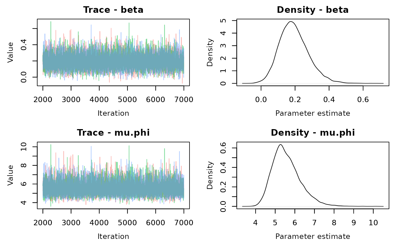
samples.time<-nimble::runMCMC(time.mcmc,
                             niter=10000,
                             nburnin = 3000,
                             nchains = 3)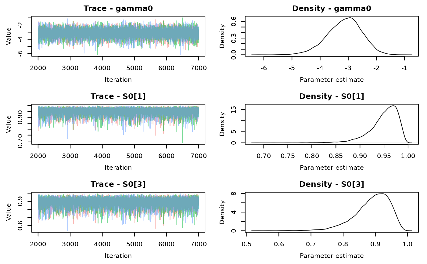

##        parm          med   dsr.med cumsurv.med
## 1   UCH0[1] 0.0450048247 0.9549952   0.9549952
## 2   UCH0[2] 0.0347043221 0.9652957   0.9202909
## 3   UCH0[3] 0.0266844750 0.9733155   0.8936064
## 23 UCH0[23] 0.0001762815 0.9998237   0.8031316
## 24 UCH0[24] 0.0001372484 0.9998628   0.8029943
## 25 UCH0[25] 0.0001070775 0.9998929   0.8028873

Analysis using logistic exposure

###########



mod.logexp<-glm(y~time,
                family=binomial(
                  link=MDChelp::logexp(glm.time.dat$exposure)),
                data=glm.time.dat)

broom::tidy(mod.logexp)->parms.logit



# parms.logit


#DSR
parms.logit%>%
  pull(estimate)->dsr.logit
# round(dsr.logit,digits=3)

age=seq(1,24,1)

dsr.logexp<-plogis(dsr.logit[1]+dsr.logit[2]*age)


# dsr.logexp

Analysis using the cloglog link and exposure time as an offset.

It turns out that this isn’t advisable when the exposure isn’t roughly the same. It gives more biased estimates. I think part of the issue to, arises from the shape of the cloglog distribution near the tails of probability. If you want hazards, just run a hazards model.

glm.time.dat$exposure



mod.clog<-glmmTMB::glmmTMB(y~time+exposure,
              family=binomial(link='cloglog'),
              data=glm.time.dat)

glmmTMB::fixef(mod.clog)$cond->parms.clog

parms.clog

age=seq(1,24,1)
median(glm.time.dat$exposure)
#offset not included because log(1) (1 exposure day) = 0

lp= parms.clog[1]+parms.clog[2]*age # linear predicator

dsr.clog=1-exp(-exp(lp))

dsr.clog

prod(dsr.clog)

State-space or HMM formulation

The last step is going to be the equivalent of what Program MARK does. It’s Bayesian so I don’t have to reformat data or anything like that because if you haven’t figured out by now, I’m kind of lazy.

##  [1] 0.9621578 0.9684107 0.9736588 0.9780547 0.9817307 0.9848006 0.9873613
##  [8] 0.9894951 0.9912719 0.9927504 0.9939799 0.9950020 0.9958512 0.9965567
## [15] 0.9971425 0.9976289 0.9980327 0.9983678 0.9986459 0.9988767 0.9990682
## [22] 0.9992271 0.9993589 0.9994682

## [1] 0.7981269

Now the fun part. The differences in the daily survival rates among different methods, compared to “Truth” (Table 4.) doesn’t seem too bad, and it’s likely due in part, to just random sampling error (this is just one realization of truth). But I would point out that the rate of change is different among the three different methods, due to their underlying distributions (exponential-hazard, modified logistic-logistic exposure, logistic-state space). This leads to some non-trivial differences in the estimates of the cumulative survival probability (Table 5.). This is a feature, not a flaw. Even going back to Shaffer 2004⁶, the daily survival estimates produced by the logistic exposure method and Program MARK are different and would lead to substantially different cumulative survival probabilities. In the example provided, the discrepancy among methods is probably also a function of the baseline survival probability and how quickly it increased. It might not be that bad if, in this case, DSR never got close to 1, increased more slowly, started lower, or the cumulative survival period was shorter.

So what to do? If I expected to model time-varying survival, I would probably use the hazard or a state-space formulation. It might seem that it’s because they seem to be the most in agreement, but it’s not. In the logistic-exposure framework, covariates are assumed to be constant across the exposure period. This is clearly not realistic if we are talking about a nest age, or other time-varying covariates we can measure even if we do not know the nest fate on the corresponding days (daily temperature, daily rainfall, etc.) These other methods however can, and I think that probably makes them a little better, across a wide range of conditions/ parameter values. That said, all models are going to be wrong, but they all are useful so do whatever works best in your situation.